Presentation of microscopy data#
Microscopy datasets are nothing more than arrays of numbers. Data can be 2D (X and Y), 5D (XYZ, Time, Color) or have even higher dimensionality. Presentation of data takes these numbers and transform them into visualizations that can be understood and analyzed by humans (as opposed to machines/algorithms). When preparing data for presentation, we keep in mind that other humans will consume it.
Colormaps#
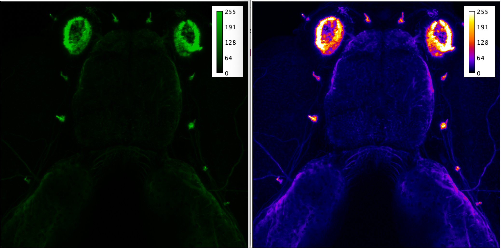
Colormaps are tools for converting numbers into pixels of specific color and intensity on the screen (or print) for human viewing. Some colormaps are better than other for human vision and screen/projector presentation, and picking best colormap depends on the way it will be viewed. In microscopy we have long-going discussions about best colormaps, and universally accepted “bad” colormaps (such as terrible default red/green/blue). Good-enough colormaps include Grayscale, Hot, Fire, and CMYK (cyan/magenta/yellow/key-black). Some colormaps are optimized for helping people with decreased color sensitivity / color-blindness. Picking the colormap might allow your listeners/readers to appreciate your effort or make them upset and angry that they can’t see anything:
Here we compare Green colormap with Fire colormap (processed in FIJI/ImageJ) on the same dataset with the same range of intensities:
Projections#
Human perception is optimized for two-dimensional datasets. Sometimes we are efficient with understanding flat images with color (3D data) but data with higher dimensionality is very difficult to consume by humans. Collapsing data along dimensions solves that problem, for example by converting 4D data (XYZ+T) into 2D (max intensity projection + temporal color-coding = XY). These projections are essentially lossy compression algorithms and generally cannot be used for quantification of datasets unless one truly understand the process by which they were created and associated limitations.
Maximum Intensity Projection#
Easiest way to collapse 3D (XYZ) datasets is to project across one of the axis using MIP (maximum intensity projection)
Color-coding in time or space#
Color-coding collapses monochrome dataset after assigning specific color to each slice. When performing on temporal dataset, it highlights pixels with specific time of change (e.g. when neurons in calcium imaging dataset “light up”), when performing in space it highlights pixels that have majority of signal at some specific location (e.g. along Z axis, thus coloring datasets by Z depth)